Nudged Elastic Band Method (NEBM)#
The NEBM is an algorithm to find minimum energy transitions between equilibrium states. This method was developed by Henkelman and Jónsson [1] to solve molecular problems in Chemistry. Later, Dittrich et al. [2] applied the NEBM to magnetic systems based on the micromagnetic theory. Recently, Bessarab et al. [3] have proposed an optimised version of the NEBM with improved control over the behaviour of the algorithm. Their review of the method allows to apply the technique to systems described by either a micromagnetic or atomistic model.
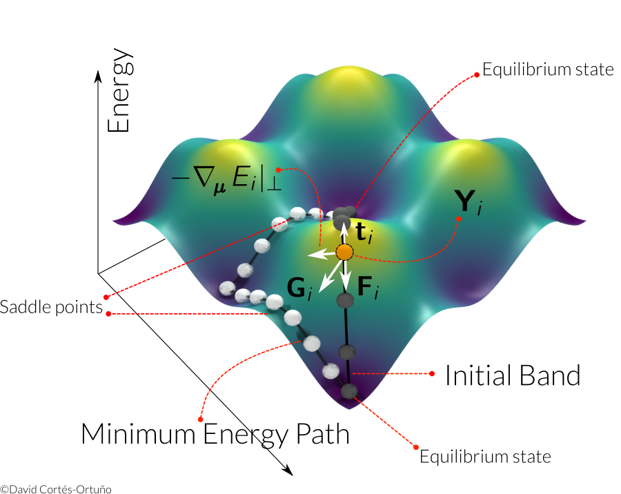
The algorithm is based on, firstly, generating \(N\) copies of a magnetic system that we describe by \(P\) spins or magnetic moments arranged in a lattice or mesh. Every copy of the system, is called an image \(\mathbf{Y}_{i}\), \(i\in \{0,\ldots,P-1\}\) and we specify an image using the spins directions in a given coordinate system. For example, in Cartesian coordinates we have
for a system described by a discrete spin model. Within the micromagnetic model we use \(\mathbf{m}\) rather than \(\mathbf{s}\), but both are unit directions.
This sequence of images defines a band, where every image is in a (ideally) different magnetic configuration. The energy of the system depends on the magnetic configuration (e.g. a skyrmion, vortex, uniform state,etc.), thus the energy is parametrised by the number of degrees of freedom, which is \(n\times P\), where \(n\) is the number of coordinates to describe a spin (e.g. \(n=3\) for Cartesian coordinates and \(n=2\) in Spherical coordinates). Accordingly, every image will have a specific energy, i.e. \(E=E(\mathbf{Y})\), which determines the position of an image in an energy landscape. The first and last images in a band are chosen as equilibrium states of the magnetic system and they are kept fixed during the NEBM evolution.
Secondly, to initiate the NEBM evolution, it is necessary to specify an initial guess for the images, which means generating different magnetic configurations between the extrema of the band. It is customary to use an interpolation of the spins directions to achieve this.
And thirdly, the band is relaxed to find a path in energy space that costs less energy. This path is characterised by passing through a saddle point, which is a maximum in energy along certain directions in phase space, and this point determines an energy barrier between the two equilibrium states. The energy barrier is the energy necessary to drive one equilibrium state towards the other. A first order saddle point is the one that is a maximum along a single direction in phase space and will usually in the energy path that costs less energy. It is possible that there are more than one energy paths.
It is also necessary to consider that:
To distinguish different images in the energy landscape we need to define a distance
To keep the images equally spaced to avoid clustering around saddle points or equilibrium states, we use a spring force between images.
Spins or magnetic moments can be described in any coordinate system. The most commonly used are spherical and Cartesian coordinates. For the later we have to specify the constraint to fix the spin length.
For a thorough explanation of the method see references [3,4].
NEBM relaxation#
Cartesian#
When using Cartesian coordinates, every image of the band \(\mathbf{Y}_{i}\) is iterated with the following dynamical equation with a fictitious time \(\tau\)
In this equation, \(\gamma\) is in units of \(\text{Hz T}^{-1}\) and it determines the time scale, which is irrelevant here so we set \(\gamma=1\). The second term to the right is necessary to keep the spins/magnetisation length equal to one, using an appropriate factor \(c\) that we set to 6. The \(\mathbf{G}\) is the total force on an image, which in the atomistic theory is defined as
and in the micromagnetic theory as
We use the magnetic effective field definition to evaluate the gradients, i.e. \(\boldsymbol{\nabla}_{\boldsymbol{\mu}}E=\partial E / (\mu_{s}\partial\mathbf{s})=-\mathbf{H}_{\text{eff}}\) or \(\boldsymbol{\nabla}_{\mathbf{M}}E=\partial E / (M_{s}\partial\mathbf{m})=-\mathbf{H}_{\text{eff}}\). The perpendicular component is with respect to the tangents \(\mathbf{t}\) to the energy band, thus for a vector \(\mathbf{A}\)
The tangents are defined according to the energies of the neighbouring images [3]. The second term to the right hand side of the equation for \(\mathbf{G}\) is the spring force that tries to keep images at equal distance and is defined using the distance between neighbouring images
which is parallel to the band, i.e. in the direction of the tangent.
According to Bessarab et al. [3], the tangents and the total force \(\mathbf{G}\) must be projected into the spin/magnetisation tangent space.
Climbing Image NEBM#
The climbing image technique is a modification of the NEBM where the forces of the image with largest energy in the band, are redefined so this image can climb up in energy along the band to get a better estimate of the saddle point energy [1,3]. The image with largest energy is chosen after relaxing the band with the usual NEBM algorithm. The total force on this climbing image is
where the spring force was removed. The climbing image is still allowed to climb down in energy in a direction perpendicular to the band, thus it is possible that the energy barrier magnitude decreases after applying this technique.
Vectors#
Following the definition of an image in Cartesian coordinates, we mentioned that the number of degrees of freedom is \(n\times P\), where \(n\) is the number of coordinates to describe a spin. Accordingly, many of the vectors in the NEBM algorithm such as the tangents, total forces, etc. have the same number of components, which agree with the spin components of an image.
For instance, the total force (or tangents, spring forces, etc.) has three components in Cartesian coordinates, corresponding to every spin direction:
Projections#
The projection of a vector into the spin/magnetisation tangent space simply means projecting its components with the corresponding spin/magnetisation field components. For example, for a vector \(\mathbf{A}\) associated to the \(i\) image of the band (we will omit the \((i)\) superscripts in the spin directions \(\mathbf{s}\) and the \(\mathbf{A}\) vector components)
the projection \(\mathcal{P}\) is defined as
where
with \(j\in\{0,\ldots,P-1 \}\), hence
Distances#
There are different ways of defining the distance in phase space between two images, \(d_{j,k}=|\mathbf{Y}_{j} - \mathbf{Y}_{k}|\).
Geodesic#
The optimised version of the NEBM [3] proposes a Geodesic distance based on Vicenty’s formulae:
where
This definition seems to work better with the NEBM since the spin directions are defined in a unit sphere.
Euclidean#
The first versions of the method simply used an Euclidean distance based on the difference between corresponding spins. In Cartesian coordinates it reads
where we have scaled the distance by the number of degrees of freedom of the system (or an image). In spherical coordinates the definition is similar, only that we use the difference of the azimuthal and polar angles and the scale is \(2P\).
Algorithm#
The algorithm can be summarised as:
Define a magnetic system and find two equilibrium states for which we want to find a minimum energy transition.
Set up a band of images and an initial sequence between the extrema. We can use linear interpolations on the spherical angles that define the spin directions [4] or Rodrigues formulae [3].
Evolve the system using the NEBM dynamical equation, which depends on the chosen coordinate system. This equation involves:
Compute the effective field for every image (they are in different magnetic configurations) and the total energy of every image
Compute the tangents according to the energies of the images and project them into the spin/magnetisation tangent space
Compute the total force for every image in the band using the tangents and distances between neighbouring images. This allows to calculate the gradient (which uses the effective field) and the spring forces on the images
Project the total force into the spin/magnetisation tangent space
Use the dynamical equation according to the coordinate system
Early versions of the NEBM did not project the vectors into the tangent space in steps I and II. This leads to an uncontrolled/poor behaviour of the band evolution since the vectors that are supposed to be perpendicular to the band still have a component along the band and interfere with the images movement in phase space.
Fidimag Code#
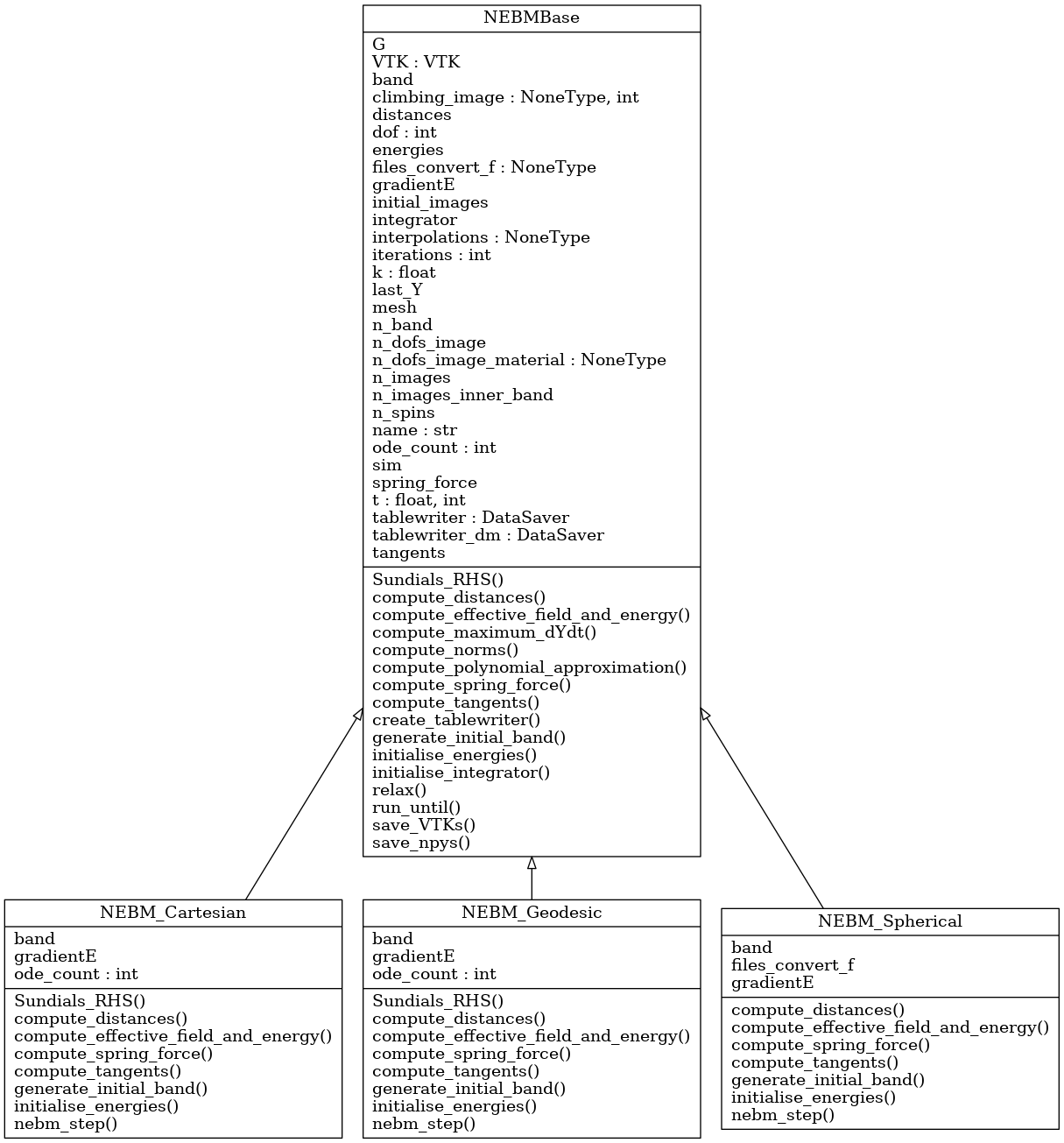
We have implemented three classes in Fidimag for the NEBM:
NEBM_Spherical: Using spherical coordinates for the spin directions and Euclidean distances with no projections into spin space. The azimuthal and polar angles need to be redefined when performing differences or computing Euclidean distances, specially because the polar angle gets undefined when it is close to the north or south. It is not completely clear what is the best approach to redefine the angles and when to do this, thus this class currently does not work properly.
NEBM_Cartesian: Using Cartesian coordinates for the spin directions and Euclidean distances with no projections into spin space. This method works well for a variety of simple system. However, when the degree of complexity increases, such as systems where vortexes or skyrmions can be stabilised, the spring force interferes with the convergence of the band into a minimum energy path. For this case it is necessary to find an optimal value of the spring constant, which is difficult since the value depends on the system size and interactions involved.
NEBM_Geodesic: Using Cartesian coordinates for the spin directions and Geodesic distances, with vectors projected in tangent space. This is the optimised version of the NEBM [3] and appears to work well with every system we have tried so far. Cartesian coordinates have the advantage that they are well defined close to the poles of the spin directions.
The following diagram shows how the code is structured:
There is a fidimag.common.nebm_tools module with common functions for the
NEBM classes:
fidimag.common.nebm_tools
|
--> cartesian2spherical
    spherical2cartesian
    compute_norm
    interpolation_Rodrigues_rotation
    linear_interpolation_spherical
Arrays#
In fidimag we mainly use Numpy to define the NEBM vectors. When calling one of
the NEBM classes, we have to pass a sim object with the specification of
the magnetic system which has associated a mesh with n_spins. According
to the coordinate system, we set the dof variable. For instance dof = 3
for Cartesian coordinates. Consequently, we define the number of degrees of
freedom per image n_dofs_image = dof * n_spins, thus if the NEBM
class was specified with n_images, the total number of degrees of freedom
for the band is n_band = n_dofs_image * n_images.
As explained in our discussion about the NEBM, we set up band,
gradientE, tangents and spring_force arrays whose length is
n_band. The order is the same than how we defined the images, thus the
Numpy array, when using Cartesian coordinates to describe the spins, looks like
band = [ s(0)_{x,0}  s(0)_{y,0}  ... s(0)_{z,n_dofs_image-1}
         s(1)_{x,0}  s(1)_{y,0}  ... s(1)_{z,n_dofs_image-1}
         ...
         s(n_images-1)_{x,0}  ... s(n_images-1)_{z,n_dofs_image-1}
       ]
and similarly for the other vectors since they follow the same order of the
spins. This band array is passed to the Cython codes to compute the NEBM
forces. Notice that we can easily redefine this array into a
(n_images, n_dofs_image) shaped Numpy array using
band = band.reshape(-1, n_dofs_image)
so every row is a different image. We can even take the inner images (no
extrema) and use the same piece of code since n_dofs_image does not change.
Cython Codes#
Most of the calculations are made using C code through Cython. The files
for these libraries are located in fidimag/common/neb_method/. Every library
has a .c file, a .h header file and a .pyx Cython file (it can
differ in name from the C files) which is compiled using Fidimag’s
setup.py file.
For example, there is a base module with common functions for every NEBM
class called nebm_lib.c
nebm_lib.c
|
--> compute_effective_force_C
    compute_norm
    compute_spring_force_C
    compute_tangents_C
    cross_product
    dot_product
    normalise
    normalise_images_C
Its corresponding header file ``nebm_lib.h contains the prototypes of these
functions. The Cython file that link some of these functions to the Python code
is called nebm_clib.pyx and can be called from the
fidimag.extensions.nebm_clib library:
fidimag.extensions.nebm_clib
|
--> compute_effective_force
    compute_tangents
The other .pyx or .c files use some of the nebm_lib.h functions.
They are separated according to the coordinate system used in the NEBM
calculations. The following diagrams show the Cython functions for these
libraries and the C files used to define them:
nebm_cartesian_lib.c
nebm_cartesian_lib.h
nebm_cartesian_clib.pyx
fidimag.extensions.nebm_cartesian_clib
|
--> compute_dYdt
    compute_effective_force
    compute_spring_force
    compute_tangents
    normalise_images
    project_images


nebm_geodesic_lib.c
nebm_geodesic_lib.h
nebm_geodesic_clib.pyx
fidimag.extensions.nebm_geodesic_clib
|
--> compute_spring_force
    geodesic_distance


nebm_spherical_lib.c
nebm_spherical_lib.h
nebm_spherical_clib.pyx
fidimag.extensions.nebm_spherical_clib
|
--> compute_spring_force
    normalise_images
Every library has its own compute_spring_force, which is taken from the
nebm_lib.c file, since the spring force depends on the
coordinate-system-dependent distance definition. For the Cartesian and
spherical coordinates, the distance functions (Euclidean distances) are not
exposed in the Cython file, as in the code for Geodesic distances.
Geodesic distances code#
Based on the aforementioned NEBM algorithm, the class initialise the NEBM calling the following methods in this order:
1. generate_initial_band   # Using linear interpolations or Rodrigues rotation formulae
|
--> nebm_tools.cartesian2spherical --> nebm_tools.linear_interpolation_spherical
    # or
    nebm_tools.interpolation_Rodrigues_rotation

2. initialise_energies     # Fill the energies array
3. initialise_integrator   # Start CVODE
4. create_tablewriter      # To pass data into .ndt files per every iteration of the integrator
The linear interpolation function requires that the input array is in spherical coordinates.
To relax the band, we use CVODE, as specified in step 3., using the
cvode.CvodeSolver (or cvode.CvodeSolver_OpenMP) integrator. The
integrator requires a Sundials_RHS function that is called on every
iteration, which is the right hand side of the \(\partial \mathbf{Y} /
\partial \tau\) dynamical equation. Correspondingly, this function
calculates the NEBM forces as
Sundials_RHS
|
--> nebm_step
    |
    --> compute_effective_field_and_energy  # Gradient = - Eff field
                                            # Which we compute for every image
                                            # using the sim class
        compute_tangents
        |
        --> nebm_clib.compute_tangents      #
            nebm_cartesian.project_images   # Project tangents
            nebm_cartesian.normalise_images #
        compute_spring_force                # Using Geodesic distances
        nebm_clib.compute_effective_force
        nebm_cartesian.project_images(G)    # Project effective (total) force

    nebm_cartesian.compute_dYdt             # Add the correction factor to fix
                                            # the spins length to 1
Many methods come from the Cartesian Cython library nebm_cartesian since
the Geodesic class uses Cartesian coordinates to describe the spins. If a
climbing image was specified as an argument for the class, we compute its
modified force in the compute_effective_force method.
The function that iterates the integrator is the relax method. On every
iteration, we compute the difference with the previous step using a scaled
Euclidean distance. The definitions of this process are specified in the
compute_maximum_dYdt method from the nebm_base class. According to the
magnitude stopping criteria specified in the stopping_dYdt argument of
relax, the iterations of the integrator will stop if the difference with
the previous step is smaller than stopping_dYdt.
Cartesian and spherical coordinates code#
These classes follow the same process than the Geodesic distances code. The
main difference is that in the nebm_step process, the projections are not
performed and the distances are computed using the scaled Euclidean distance.
Spherical#
For spherical coordinates, the vectors are smaller, with n_dofs_image = 2 * n_spins,
where
band = [ theta(0)_{0}  phi(0)_{0} theta(0)_{1} ... phi(0)_{n_dofs_image-1}
         theta(1)_{0}  phi(1)_{0} theta(1)_{1} ... phi(1)_{n_dofs_image-1}
         ...
         theta(n_images-1)_{0} ... phi(n_images-1)_{n_dofs_image-1}
       ]
The Sundials_RHS function does not include the correction factor since
spherical coordinates have implicit the constraint of fixed length for the
magnetisation. When computing distances or differences, it is necessary to
redefine the angles, but it is not completely clear the optimal way of doing
this.